How to Remove Duplicates in Excel (Step-by-Step Guide)

Duplicate data is one of the most common headaches in Excel  if it’s from copy-pasting between sheets, merging data from multiple sources, or repeated form submissions. Left unchecked, duplicates can throw off your totals, skew reports, and make even simple formulas return misleading results.

The good news is that Excel gives you several reliable ways to find and remove duplicates, and you don’t need advanced skills to use them. If you want a quick one-click cleanup, a safer method that highlights duplicates before deleting anything, or more control using formulas and PivotTables, there’s an approach that fits your situation.

In this guide, we’ll walk through the built-in Remove Duplicates tool, conditional formatting, formula-based methods, and a few bonus tips to help you avoid common mistakes along the way.

Understanding Duplicates in Excel

Before removing anything, it’s worth understanding what actually counts as a “duplicate” in Excel  because the definition isn’t always as simple as it sounds.

At the most basic level, a duplicate is a row where every value across all selected columns matches another row exactly. But in real-world spreadsheets, duplicates are often more nuanced. For example, two rows might have the same customer name but different email addresses, or the same order ID but slightly different formatting (extra spaces, different capitalization). Excel treats these as separate cases depending on which columns you check and how strictly you define a “match.”

This distinction matters because duplicates can cause real problems in your data:

• Skewed reports: Duplicate entries can inflate totals, averages, and counts, leading to inaccurate summaries.
• Broken formulas: Functions like SUM, COUNT, or VLOOKUP may return incorrect results if they’re pulling from duplicated rows.
• Data integrity issues: Duplicate customer records, transactions, or inventory entries can create confusion across teams relying on the same spreadsheet.

Duplicates typically creep into spreadsheets through a few common causes: manual copy-paste errors, importing data from multiple sources (like combining exports from different systems), repeated form submissions, or accidentally pasting the same dataset twice.

Understanding the type of duplicate you’re dealing with  exact row matches versus partial matches on specific columns  will help you choose the right removal method in the sections ahead, rather than applying a one-size-fits-all fix that might delete data you actually need.

Before You Start: Preparation Tips

Removing duplicates is one of the few Excel actions that can permanently alter your data, so a little preparation goes a long way before you touch anything.

Always back up your data first. Before running any duplicate-removal method, copy your original data to a new sheet or save a separate copy of the file. This gives you a safety net in case the wrong rows get deleted or you need to reference the original dataset later.

Use Excel Tables for cleaner referencing. Converting your data range into an Excel Table (Insert > Table) makes it easier to apply formulas, filters, and formatting consistently, and helps prevent errors caused by accidentally selecting the wrong range.

Freeze your header row. If you’re scrolling through a large dataset, freezing the header row (View > Freeze Panes) keeps column labels visible, reducing the risk of misidentifying which column you’re working with.

Decide your goal before choosing a method. Ask yourself: do you want to permanently delete duplicate rows, or simply identify and review them first? These require different approaches; the built-in Remove Duplicates tool deletes data immediately, while conditional formatting or formulas let you flag duplicates without touching the original dataset.

Check for inconsistent formatting. Extra spaces, inconsistent capitalization, or mismatched date formats can cause Excel to treat identical-looking entries as different values (or vice versa). Cleaning up formatting beforehand helps ensure your duplicate check is accurate.

Taking these steps first can save significant time  and prevent accidental data loss  before diving into the removal methods below.

Method 1: Using “Remove Duplicates” Tool (Built-In Feature)

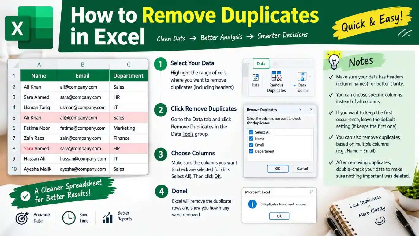
Excel’s built-in Remove Duplicates tool is the fastest way to clean up duplicate data, and it’s ideal when you’re confident about which rows you want to delete.

Step-by-step walkthrough:

1. Select your data range, or click anywhere inside your dataset if it’s formatted as a Table.
2. Go to the Data tab on the ribbon.
3. Click Remove Duplicates in the Data Tools group.
4. A dialog box will appear listing all your columns with checkboxes. If your data has headers, make sure “My data has headers” is checked.
5. Choose if to check all columns (for exact row matches) or only specific columns (for partial matches, like duplicate emails regardless of other differences).
6. Click OK. Excel will remove duplicate entries and show a summary of how many duplicate values were found and removed, along with how many unique values remain.

Selecting specific columns vs. entire rows:
If you only check certain columns, Excel treats any row with matching values in those columns as a duplicate  even if other columns differ. This is useful when you only care about uniqueness in key fields, like customer ID or email address.

Important caution:
This method permanently deletes duplicate rows as soon as you click OK. There’s no built-in preview, so make sure you’ve backed up your data first (as covered in the previous section).

Best use case: Quick, straightforward cleanup when you’re confident about your criteria and have already backed up your file.

Method 2: Highlighting Duplicates with Conditional Formatting

If you’re not ready to delete anything yet, conditional formatting is a safer way to spot duplicates visually before taking action. Unlike the Remove Duplicates tool, this method doesn’t touch your original data; it simply highlights matching values so you can review them first.

Step-by-step walkthrough:

1. Select the range of cells you want to check for duplicates.
2. Go to the Home tab on the ribbon.
3. Click Conditional Formatting in the Styles group.
4. Hover over Highlight Cell Rules, then select Duplicate Values.
5. In the dialog box, choose a formatting style (Excel offers preset colors like light red fill with dark red text, or you can customize your own).
6. Click OK. Excel will instantly highlight any cells with duplicate values within your selected range.

You can also reverse this to highlight unique values instead, which is useful when you want to see what’s left after removing duplicates without actually deleting anything yet.

Why this method is safer:
Because conditional formatting only changes the appearance of cells rather than deleting data, it gives you a clear visual overview of duplicates before deciding how to handle them. This is especially useful for spotting patterns  like duplicates clustered in a specific section of your data, which might indicate a larger import or entry error.

Best use case: Reviewing and auditing data before deletion, or when you want an ongoing visual check as new data is added to the sheet.

Method 3: Using COUNTIF/COUNTIFS to Identify Duplicates

For more control over how duplicates are identified, especially when you want to keep the first occurrence and only flag the rest, formulas like COUNTIF and COUNTIFS offer a flexible alternative to Excel’s built-in tools.

Basic COUNTIF formula:
To flag duplicates in a single column, add a helper column next to your data and use:

=COUNTIF(A:A, A2)>1

This checks how many times the value in cell A2 appears in column A. If it appears more than once, the formula returns TRUE, flagging it as a duplicate.

Identifying duplicates across multiple columns with COUNTIFS:
If you need to check for duplicates based on more than one column (for example, matching both first and last name), use:

=COUNTIFS(A:A, A2, B:B, B2)>1

This only flags a row as duplicate if both column A and column B match another row.

Keeping only the first occurrence:
A common need is identifying duplicates while keeping the first instance untouched. You can do this with:

=COUNTIF($A$2:A2, A2)>1

Using a mixed reference (locking the starting row) means Excel only counts occurrences up to the current row, so the first instance returns FALSE while any repeats after it return TRUE.

Once flagged, you can filter by TRUE values in the helper column and delete, review, or export those rows as needed.

Best use case: When you need more precision than the built-in tool offers, such as keeping the first occurrence, checking multiple columns together, or building a repeatable, auditable process.

Method 4: Using Advanced Filter for Unique Records

If you want to extract a clean list of unique values without altering your original dataset, Excel’s Advanced Filter tool is one of the most underused but effective options available.

Step-by-step walkthrough:

1. Select your data range, including headers.
2. Go to the Data tab on the ribbon.
3. Click Advanced in the Sort & Filter group (this opens the Advanced Filter dialog).
4. Choose “Copy to another location” if you want to keep your original data untouched and generate a separate unique list. Choose “Filter the list, in-place” if you’d rather just filter the current view.
5. Set your List range (your original data) and, if copying elsewhere, set the Copy to field to specify where the unique list should appear.
6. Check the box labeled “Unique records only.”
7. Click OK. Excel will generate a list containing only unique rows, leaving duplicates out entirely.

Difference from Remove Duplicates:
Unlike the Remove Duplicates tool, which deletes duplicate rows directly from your original data, Advanced Filter can create a brand-new list elsewhere, leaving your source data completely intact. This makes it a safer option when you need a clean dataset for reporting or export, but still want to preserve the raw data for reference.

Best use case: Generating a duplicate-free list for reports, exports, or further analysis, without permanently modifying your original spreadsheet, especially useful when multiple people rely on the same source file.

Method 5: Using PivotTables to Find Duplicates

PivotTables aren’t typically thought of as a duplicate-removal tool, but they’re one of the best ways to quickly surface how often values repeat across a large dataset, especially when you’re more interested in identifying patterns than just deleting rows.

Step-by-step walkthrough:

1. Select your data range, including headers.
2. Go to the Insert tab and click PivotTable.
3. Choose where you’d like the PivotTable placed (a new worksheet is usually easiest).
4. In the PivotTable Field List, drag the column you want to check for duplicates (e.g., “Customer Name” or “Order ID”) into both the Rows area and the Values area.
5. In the Values area, make sure the field is set to Count rather than Sum.
6. Review the resulting table  any value with a count greater than 1 indicates a duplicate entry.

You can also add a filter to only display values with a count greater than one, giving you an instant list of exactly which entries are duplicated and how many times each appears.

Why this method works well for large datasets:
Rather than scanning thousands of rows manually or relying on conditional formatting alone, a PivotTable summarizes the entire dataset at a glance, making it easy to spot which values are duplicated most frequently  useful for identifying data entry patterns or recurring errors at the source.

Best use case: Large datasets where you need a summarized overview of duplicate frequency, rather than just a simple flag or deletion.

Removing Duplicates Based on Specific Columns Only

Not every duplicate needs to match across an entire row  often, you only care about uniqueness in one or two key columns, while other columns are allowed to differ. Handling this correctly requires a slightly different approach than a full-row duplicate check.

A common example:
Imagine a customer list where two rows share the same name, but have different email addresses. If you check for duplicates across all columns, Excel won’t flag these as duplicates, since the email column differs. But if your goal is to ensure each customer name appears only once  regardless of what’s in other columns  you need to base the check on that specific column alone.

How to handle this in the Remove Duplicates tool:
When the Remove Duplicates dialog box appears, uncheck all columns except the one(s) you want to base the match on (for example, just “Customer Name”). Excel will then treat any row with a matching value in that column as a duplicate, even if the rest of the row differs  and it will keep only the first occurrence, deleting the rows that follow.

A note on accuracy:
Before doing this, make sure you’re confident that matches in the selected column truly represent duplicate records, and not simply coincidental repeats (like two different customers who happen to share the same name). When in doubt, cross-check with a secondary identifier, such as an email address or customer ID, using the COUNTIFS method from the previous section.

Column selection strategy: Always start with the most specific, least ambiguous column, such as an ID field, before relying on names or categories that might repeat naturally.

Common Mistakes to Avoid

Even with the right tools, a few common mistakes can lead to lost data or duplicates that don’t get properly removed. Watching out for these can save significant cleanup time later.

Not backing up data first. This is the single most important step to skip at your own risk. The Remove Duplicates tool deletes rows permanently and offers no built-in undo beyond Excel’s standard Ctrl+Z, which won’t help if you’ve already saved and closed the file. Always keep a backup copy before running any duplicate removal.

Selecting the wrong columns or range. Accidentally including or excluding a column in the Remove Duplicates dialog can lead to either too many rows being deleted or duplicates being missed entirely. Double-check your column selection before clicking OK.

Extra spaces and inconsistent formatting. Values that look identical  like “John Smith” and “John Smith ” (with a trailing space)  may be treated as different entries because Excel checks for exact matches. Similarly, inconsistent capitalization or date formats can cause duplicates to slip through undetected. Running a TRIM formula beforehand can help catch these issues.

Case sensitivity assumptions. By default, Excel’s Remove Duplicates tool is not case-sensitive, meaning “Smith” and “SMITH” are treated as duplicates. If case matters for your dataset, you’ll need a formula-based approach instead.

Merged cells breaking the tool. Merged cells can cause unexpected behavior or errors when using Remove Duplicates or Advanced Filter. It’s best to unmerge cells before attempting any duplicate-removal process.

Avoiding these pitfalls helps ensure your duplicate cleanup is accurate  and that you don’t lose data you actually needed to keep.

FAQs

Does Remove Duplicates delete the first or second occurrence?
Excel’s Remove Duplicates tool always keeps the first occurrence of a duplicate value (based on the order rows appear in your sheet) and deletes any subsequent matches. If row order matters, sort your data first to control which entry is treat as the “original.”

Can I undo Remove Duplicates?
Yes, but only immediately after running it. Pressing Ctrl+Z right away will restore the deleted rows. However, if you’ve closed the file, saved changes, or performed other actions afterward, the undo history may no longer be available  which is why backing up your data beforehand is so important.

How do I remove duplicates but keep one copy?
This is exactly what the Remove Duplicates tool does by default: it automatically keeps the first occurrence of each duplicate and removes the rest. No additional settings are being needed for this behavior.

Does this work in Google Sheets the same way?
Google Sheets has a similar “Remove duplicates” feature under the Data menu, and it functions almost identically. However, formula-based approaches (like COUNTIF or UNIQUE) may have slightly different syntax or behavior between the two platforms, so it’s worth double-checking formulas when switching between them.

Why isn’t removing duplicates catching all duplicates?
This usually happens due to inconsistent formatting, extra spaces, mismatched capitalization, or different date/number formats can cause Excel to treat visually identical values as different. Cleaning your data with TRIM, UPPER/LOWER, or consistent formatting beforehand usually resolves this.

Conclusion

Duplicate data is one of the most common issues in Excel, but as this guide shows, there’s no shortage of ways to handle it  if you want a quick one-click fix or a more careful, formula-driven approach. The built-in Remove Duplicates tool is fast and effective for straightforward cleanups, while conditional formatting offers a safer way to review duplicates visually before deleting anything. For more control, COUNTIF and COUNTIFS formulas let you flag duplicates based on specific criteria, including keeping only the first occurrence or checking multiple columns at once.

For situations where you need to preserve your original dataset, Advanced Filter and PivotTables provide reliable ways to extract unique records or analyze duplicate frequency without altering your source data. And when duplicates only matter within certain columns  like a customer name or ID, adjusting your column selection ensures you’re not accidentally deleting valid, unique records.